8 install.packages(‘gutenbergr’)

#Text Analysis

Let’s use our text analysis on works on literature - we’ll look for patterns in the greatest works by Dostoevsky, but feel free to use the same technique to explore any other author or text.

Keep in mind, the more text content you analyze, the more accurate your overall results should be. If I looked at the three greatest books by Dostoevsky, I’d potentially find a lot - but my methodology would only allow for me to apply those results to a conclusion on those three books, not any others - much less all of an author’s work. If I want to make grand claims about how Dostoevsy writes, I need to analyze as much of his work as possible. Ideally, we could set a high bar for primary information, which others could also use if duplicating our research: something like the ‘10 most popular books by Dostoevsky.’ How would we determine that?

Feodor Dostoevsky wrote 11 novels in his life, and five seem to be recognized as his greatest works, according to many lists online. Do we analyze all 11, or just the 5 ‘best?’ Do we include his short stories and novellas? Again, the more data the better - and also, after initially loading the data, there’s really no extra work involved in adding more books to the project. So add them.

And why Dostoevsky? Why no analyze the Harry Potter books? Well, Feodor is dead, and his works are in the public domain - which means we can connect to the website gutenberg.org and download copies of his books for free. We can’t do that with Harry Potter, as those books are copyrighted. We could still attempt to find and load that data, but chances are it’d be very messy and hard to analyze if someone did the text conversion themselves. In the case of very popular works like Harry Potter or Hamilton, megafans have created clean data for text analysis and posted it on GitHub. But I’ll stick with Dostoevsky.

If you explore gutenberg.org, you’ll find hundreds of books in the public domain available for download. Each book has a number associated with it, most easily found in the URL when looking at a particular novel. I’m going to load Dostoevsky’s books using the Gutenbergr package and these numbers.

library(tidyverse)
library(gutenbergr)

gutenberg_works(author == "Dostoyevsky, Fyodor")

# A tibble: 14 × 8
   gutenberg_id title    author gutenberg_author_id language gutenberg_bookshelf
          <int> <chr>    <chr>                <int> <fct>    <chr>              
 1          600 "Notes … Dosto…                 314 en       Category: Novels/C…
 2         2197 "The Ga… Dosto…                 314 en       Category: Novels/C…
 3         2302 "Poor F… Dosto…                 314 en       Category: Novels/C…
 4         2554 "Crime … Dosto…                 314 en       Best Books Ever Li…
 5         2638 "The Id… Dosto…                 314 en       Best Books Ever Li…
 6         8117 "The po… Dosto…                 314 en       Best Books Ever Li…
 7         8578 "The Gr… Dosto…                 314 en       Racism/Category: P…
 8        28054 "The Br… Dosto…                 314 en       Best Books Ever Li…
 9        36034 "White … Dosto…                 314 en       Category: Short St…
10        37536 "The ho… Dosto…                 314 en       Category: Novels/C…
11        38241 "Uncle'… Dosto…                 314 en       Category: Short St…
12        40745 "Short … Dosto…                 314 en       Category: Short St…
13        57050 "Stavro… Dosto…                 314 en       Category: Novels/C…
14        59196 "Index … Dosto…                 314 en       Category: Russian …
# ℹ 2 more variables: rights <fct>, has_text <lgl>

OK, there they are! While there are 12 results, not all of them are novels - we also have some short story collections. Let’s include them all, and to make sure we do, here’s an index of all Dostoevsky books on gutenberg.org:

Project Gutenberg: Dostoevsky

Now to download them as .txt files. Note that I use the ‘mutate’ function of dplyr to add a column with the name of each book - this is so, when we merge all of the books together into one big ‘corpus,’ we can still figure out which book the text came from.

This is a lot of code, but we’re just loading all of these books into R: lots of repetition.

crime <- gutenberg_download(2554, mirror = "http://mirrors.xmission.com/gutenberg/") |> 
  mutate('title' = "Crime & Punishment")

brothers <-gutenberg_download(28054, mirror = "http://mirrors.xmission.com/gutenberg/") |> 
  mutate('title' = "The Brothers Karamazov")

notes <-gutenberg_download(600, mirror = "http://mirrors.xmission.com/gutenberg/") |> 
  mutate('title' = "Notes from the Underground")

idiot <-gutenberg_download(2638, mirror = "http://mirrors.xmission.com/gutenberg/") |> 
  mutate('title' = "The Idiot")

demons <-gutenberg_download(8117, mirror = "http://mirrors.xmission.com/gutenberg/") |> 
  mutate('title' = "The Possessed")

gambler <-gutenberg_download(2197, mirror = "http://mirrors.xmission.com/gutenberg/") |> 
  mutate('title' = "The Gambler")

 poor <-gutenberg_download(2302, mirror = "http://mirrors.xmission.com/gutenberg/") |> 
   mutate('title' = "Poor Folk")
 
 white <-gutenberg_download(36034, mirror = "http://mirrors.xmission.com/gutenberg/") |> 
   mutate('title' = "White Nights and Other Stories")
 
 house <-gutenberg_download(37536, mirror = "http://mirrors.xmission.com/gutenberg/") |> 
   mutate('title' = "The House of the Dead")
 
 uncle <-gutenberg_download(38241, mirror = "http://mirrors.xmission.com/gutenberg/") |> 
   mutate('title' = "Uncle's Dream; and The Permanent Husband")
 
 short <-gutenberg_download(40745, mirror = "http://mirrors.xmission.com/gutenberg/") |> 
   mutate('title' = "Short Stories")
 
 grand <-gutenberg_download(8578, mirror = "http://mirrors.xmission.com/gutenberg/") |> 
   mutate('title' = "The Grand Inquisitor")
 
 stavrogin <-gutenberg_download(57050, mirror = "http://mirrors.xmission.com/gutenberg/") |> 
   mutate('title' = "Stavrogin's Confession and The Plan of The Life of a Great Sinner")

8.1 Creating a Corpus

Now, let’s merge all of the books into one huge corpus (a corpus is a large, structured collection of text data). We’ll do this using the function rbind(), which is the easiest way to merge data frames with identical columns, as we have here.

dostoyevsky <- rbind(crime,brothers, notes, idiot, demons, gambler, poor, white, house, uncle, short, grand, stavrogin)

8.2 Finding Common Words

So, what are the most common words used by Dostoevsky?

To find out, we need to change this data frame of literature into a new format: one that has one-word-per-row. In other words, for every word of every book, we will have a row of the data frame that indicates the word and the book the word is from. We can then calculate things like the total number of instances of a word, and the like.

This process is called tokenization, as a word is only one potential token to analyze (others include letters, bigrams, sentences, paragraphs, etc.). We tokenize our words using the tidytext package, a companion to teh tidyverse that specifically works with text data.

To tokenize our text into words, we’ll use the unnest_tokens() function of the tidytext package. Inside the function, ‘word’ indicates the token we’re specifying, and ‘text’ is the name of the column that currently contains all of the words from the books. We’ll create a new data frame called ‘d_words.’

#install.packages('tidytext')
library(tidytext)

dostoyevsky |> 
  unnest_tokens(word, text) -> d_words

If we were to look at the most common words now - d_words |> count(word, sort = TRUE) - we’d see a lot of words like ‘the, and, of’ - what we call ‘stop words.’ Let’s remove those, as they give no indication of emotion, and their relative frequency is uninteresting.

The tidytext package already has a lexicon of stop words that we can use for this purpose. To remove them from our corpus, we’ll perform an anti-join, which is when you merge two data frames but only keep the content that does not show up in both. All of the stop words will show up in both stop_words and d_words, and will be taken out. And then let’s count the most frequent words:

d_words |> 
  anti_join(stop_words) |> 
#  group_by(title) |> 
  count(word, sort = TRUE) |> 
  head(20) |> 
  knitr::kable()

Joining with `by = join_by(word)`

word	n
time	3291
day	2245
prince	2243
suddenly	2111
don’t	1912
cried	1828
eyes	1692
life	1603
looked	1596
people	1582
moment	1566
it’s	1525
love	1389
money	1373
heart	1347
house	1286
hand	1274
understand	1204
told	1196
alyosha	1194

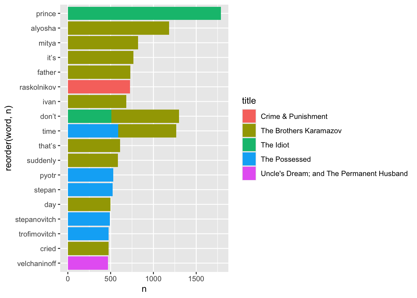
We could visualize this, but it’d be a pretty boring and uninformative bar chart. What could make it more interesting is if we kept the data on which book the words show up in.

d_words |> 
  anti_join(stop_words) |> 
  group_by(title) |> 
  count(word, sort = TRUE) |> 
  head(20) |> 
  ggplot(aes(reorder(word, n),n, fill = title)) + geom_col() + coord_flip()

Joining with `by = join_by(word)`

8.3 Bigrams

Bigrams are just collections of words that show up next to each other in a text, like ‘United States’ or ‘ice cream.’ When we count bigrams, we can also measure what word or words most frequently precedes or comes after another word. For instance, Lewis Carrol’s relative disdain for his protagonist Alice is clear when performing a bigram analysis of what words come before her name: the most frequent is poor, as in poor Alice.

To generate bigrams, we have to re-tokenize our text:

#bigrams!
dostoyevsky |> 
  unnest_tokens(bigram, text, token="ngrams", n=2) -> d_bigrams

While that creates bigrams, they are grouped together in one column of the data frame, so we can’t measure them independently.

Let’s use dplyr’s separate() function to split them into two columns:

 d_bigrams |> 
   separate(bigram, c("word1", "word2"), sep = " ") -> d_bigrams

We couldn’t previously remove stop words, as we’d change the order of what words follow each other in the text - rendering a bigram analysis riddled with errors. But now that our words have been collected as bigram pairs, we can remove any with stop words or NAs, or blanks:

d_bigrams |>  
  filter(!word1 %in% stop_words$word) |>
  filter(!word2 %in% stop_words$word) |> 
  filter(!word1 %in% NA) |> 
  filter(!word2 %in% NA) -> d_bigrams

Now let’s count the most common bigrams - kind of predictable results.

d_bigrams |> 
count(word1, word2, sort = TRUE)

# A tibble: 81,386 × 3
   word1    word2               n
   <chr>    <chr>           <int>
 1 pyotr    stepanovitch      431
 2 stepan   trofimovitch      406
 3 varvara  petrovna          340
 4 katerina ivanovna          310
 5 pavel    pavlovitch        283
 6 nikolay  vsyevolodovitch   247
 7 ha       ha                241
 8 fyodor   pavlovitch        215
 9 maria    alexandrovna      214
10 nastasia philipovna        183
# ℹ 81,376 more rows

What’s more productive is to search for the most common words to come just before or after another word. For instance, what are the most common words to precede ‘fellow?’

d_bigrams |>  
  filter(word2 == "fellow")

# A tibble: 286 × 4
   gutenberg_id title              word1    word2 
          <int> <chr>              <chr>    <chr> 
 1         2554 Crime & Punishment funny    fellow
 2         2554 Crime & Punishment funny    fellow
 3         2554 Crime & Punishment crazy    fellow
 4         2554 Crime & Punishment crazy    fellow
 5         2554 Crime & Punishment low      fellow
 6         2554 Crime & Punishment capital  fellow
 7         2554 Crime & Punishment rate     fellow
 8         2554 Crime & Punishment boastful fellow
 9         2554 Crime & Punishment nice     fellow
10         2554 Crime & Punishment dear     fellow
# ℹ 276 more rows

That’s a little more interesting.

8.4 Word Clouds

It’s very easy to generate a word cloud from a very specific data frame: one with the columns ‘word’ and ‘n,’ showing word frequency. Your data frame can have other columns in it, but it needs these two in particular - and they have to be named correctly, too.

The version of wordcloud on CRAN has been riddled with an error for some time, so let’s install the development version from GitHub. In order to do this, we need to add the devtools package.

install.packages('devtools')
library(devtools)
devtools::install_github('lchiffon/wordcloud2')

Let’s make a word cloud without the stop_words:

library(wordcloud2)

d_words |> 
  anti_join(stop_words) |> 
  count(word, sort = TRUE) |> 
  wordcloud2()

Joining with `by = join_by(word)`

8.5 Sentiment

For our final analysis, we can measure sentiment from the three sentiment lexicons built into the tidytext package. They are:

Bing, for providing simple (boolean) positive/negative values of TRUE or FALSE
NRC, for assigning emotions to words beyond just positive & negative - such as trust, surprise, joy & disgust
AFINN, which ranks a word’s sentiment on a scale that goes from -5 to 5, with neutral words at 0

In order to use AFINN, we need to load one additional package:

install.packages('textdata')
library(textdata)

To measure sentiment, we will once again join our data to a lexicon. In this case, we want to perform an inner_join, which is essentially the opposite of an anti_join: keep only the words that show up in both locations. As a result, we’ll throw away all of the words in the text that do not have a sentiment value.

Let’s start with Bing.

d_words |> 
  anti_join(stop_words) |> 
  inner_join(get_sentiments("bing")) |> 
  group_by(sentiment) |> 
  count() |> 
  knitr::kable()

Joining with `by = join_by(word)`
Joining with `by = join_by(word)`

Warning in inner_join(anti_join(d_words, stop_words), get_sentiments("bing")): Detected an unexpected many-to-many relationship between `x` and `y`.
ℹ Row 26135 of `x` matches multiple rows in `y`.
ℹ Row 4651 of `y` matches multiple rows in `x`.
ℹ If a many-to-many relationship is expected, set `relationship =
  "many-to-many"` to silence this warning.

sentiment	n
negative	63879
positive	35217

There seem to be a lot more negative words than positive ones. Let’s see what some of these words are, ranked by their sentiment score - which is a part of AFINN:

d_words |> 
  anti_join(stop_words) |> 
  inner_join(get_sentiments("afinn")) |> 
  group_by(value) |> 
  count(word, sort=TRUE) |> 
  head(12) |> 
  knitr::kable()

Joining with `by = join_by(word)`
Joining with `by = join_by(word)`

value	word	n
-2	cried	1828
3	love	1389
1	god	1013
2	dear	852
1	matter	778
-1	strange	747
-2	poor	730
-2	afraid	700
2	true	649
1	feeling	633
-1	leave	555
-2	tears	550

How about using Bing to measure the positivity / negativity of each book?

d_words |> 
  anti_join(stop_words) |> 
  inner_join(get_sentiments("bing")) |> 
  group_by(title) |> 
  count(sentiment, sort=TRUE) |> 
  knitr::kable()

Joining with `by = join_by(word)`
Joining with `by = join_by(word)`

Warning in inner_join(anti_join(d_words, stop_words), get_sentiments("bing")): Detected an unexpected many-to-many relationship between `x` and `y`.
ℹ Row 26135 of `x` matches multiple rows in `y`.
ℹ Row 4651 of `y` matches multiple rows in `x`.
ℹ If a many-to-many relationship is expected, set `relationship =
  "many-to-many"` to silence this warning.

title	sentiment	n
The Brothers Karamazov	negative	14083
The Possessed	negative	9492
The Idiot	negative	8361
Crime & Punishment	negative	8257
The Brothers Karamazov	positive	7903
The Idiot	positive	4943
The Possessed	positive	4936
White Nights and Other Stories	negative	4840
The House of the Dead	negative	4733
Uncle’s Dream; and The Permanent Husband	negative	3578
Crime & Punishment	positive	3453
Short Stories	negative	2957
White Nights and Other Stories	positive	2945
The House of the Dead	positive	2618
Uncle’s Dream; and The Permanent Husband	positive	2308
Poor Folk	negative	2085
Notes from the Underground	negative	2053
Short Stories	positive	1777
The Gambler	negative	1775
Stavrogin’s Confession and The Plan of The Life of a Great Sinner	negative	1250
Poor Folk	positive	1179
Notes from the Underground	positive	1103
The Gambler	positive	1078
Stavrogin’s Confession and The Plan of The Life of a Great Sinner	positive	630
The Grand Inquisitor	negative	415
The Grand Inquisitor	positive	344

OK, and let’s see at what NRC looks like:

d_words |> 
  anti_join(stop_words) |> 
  inner_join(get_sentiments("nrc")) |> 
  # group_by(title) |> 
  count(sentiment,  sort=TRUE)

Joining with `by = join_by(word)`
Joining with `by = join_by(word)`

Warning in inner_join(anti_join(d_words, stop_words), get_sentiments("nrc")): Detected an unexpected many-to-many relationship between `x` and `y`.
ℹ Row 1 of `x` matches multiple rows in `y`.
ℹ Row 10122 of `y` matches multiple rows in `x`.
ℹ If a many-to-many relationship is expected, set `relationship =
  "many-to-many"` to silence this warning.

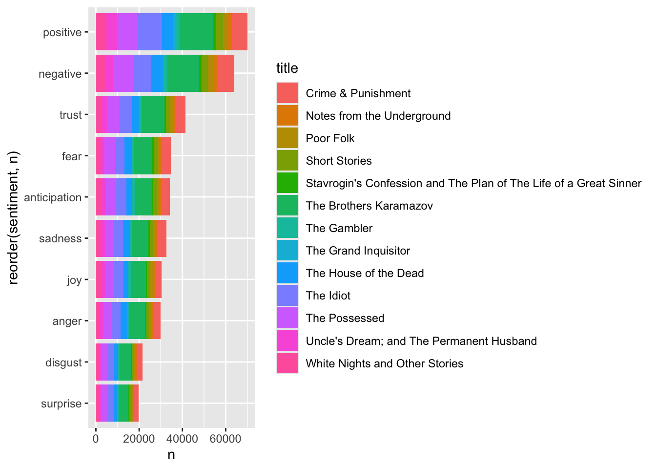
# A tibble: 10 × 2
   sentiment        n
   <chr>        <int>
 1 positive     70008
 2 negative     64048
 3 trust        41304
 4 fear         34710
 5 anticipation 34137
 6 sadness      32716
 7 joy          30247
 8 anger        29819
 9 disgust      21617
10 surprise     19801

These can all be plotted, of course:

d_words |> 
  anti_join(stop_words) |> 
  inner_join(get_sentiments("nrc")) |> 
   group_by(title) |> 
  count(sentiment, sort=TRUE) |> 
  ggplot(aes(reorder(sentiment, n),n, fill = title)) + geom_col() + coord_flip()

Joining with `by = join_by(word)`
Joining with `by = join_by(word)`

Warning in inner_join(anti_join(d_words, stop_words), get_sentiments("nrc")): Detected an unexpected many-to-many relationship between `x` and `y`.
ℹ Row 1 of `x` matches multiple rows in `y`.
ℹ Row 10122 of `y` matches multiple rows in `x`.
ℹ If a many-to-many relationship is expected, set `relationship =
  "many-to-many"` to silence this warning.

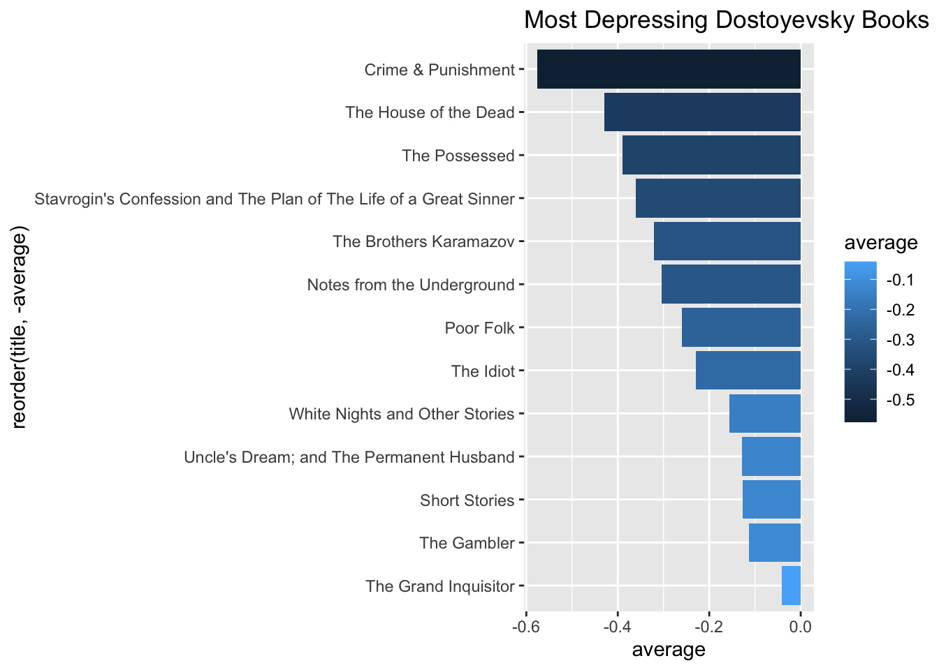
So, what are the most depressing Dostoevsky books? Let’s use AFINN to calculate a mean for the sentiment value per book:

d_words |> 
  anti_join(stop_words) |> 
  inner_join(get_sentiments("afinn")) |> 
  group_by(title) |> 
  #count(word, value, sort=TRUE) |> 
  summarize(average = mean(value)) |> 
  ggplot(aes(reorder(title, -average), average, fill=average)) + geom_col() + coord_flip() +
  ggtitle("Most Depressing Dostoyevsky Books")

Joining with `by = join_by(word)`
Joining with `by = join_by(word)`